Toy simulations
So far we have used asymptotic formulae to compute
p-values and define confidence regions. As explained in Statistical inference, the
asymptotic formulae hold exactly only for linear regression models. Since the model in our
examples is non-linear this is at best an approximation. To test the quality of
this approximation we have to generate toy observables  distributed according to the PDF
  of our model for some parameter vector
  , and
determine the distribution of
, and
determine the distribution of  . This is called a
toy simulation. If the asymptotic formulae are applicable the
. This is called a
toy simulation. If the asymptotic formulae are applicable the
 should have a chi-square distribution with
 degrees of freedom.
If asymptotic formulae are not applicable you can use toy simulations to compute
the (plug-in) p-value numerically. To do this you
simply count the fraction of toy observable vectors  for which
 , where
  is
the observed data. If the p-value is small you need a large number of toy
observables to estimate this fraction with a reasonable accuracy. For example,
to claim “3 sigma evidence” for something you have to show that the p-value is
smaller than
is
the observed data. If the p-value is small you need a large number of toy
observables to estimate this fraction with a reasonable accuracy. For example,
to claim “3 sigma evidence” for something you have to show that the p-value is
smaller than  . To estimate such a small p-value with a
(relative) 10% accuracy you need about 40000 toys. For a “5 sigma discovery” you
alread need
. To estimate such a small p-value with a
(relative) 10% accuracy you need about 40000 toys. For a “5 sigma discovery” you
alread need  toys. Simulating such a large number of toys
is often impossible, even with a computing cluster. Remember that computing the
for one toy vector requires two numerical
optimisations which, for difficult problems, can take several seconds.
toys. Simulating such a large number of toys
is often impossible, even with a computing cluster. Remember that computing the
for one toy vector requires two numerical
optimisations which, for difficult problems, can take several seconds.
myFitter implements an improved method for numerical p-value computations which
is based on importance sampling (and referred to as myFitter method in the
following). It exploits “geometric” information about the parameter spaces
 and
and  to generate toys which are more likely to
give a larger than
to generate toys which are more likely to
give a larger than  . The
details are explained in arXiv:1207.1446,
but you don’t need to know them in order to use the method. This section shows
you how.
. The
details are explained in arXiv:1207.1446,
but you don’t need to know them in order to use the method. This section shows
you how.
The myFitter class which is responsible for running toy simulations and computing p-values (both with the standard and the myFitter method) is called ToySimulator. Since numerical p-value computations are essentially multi-dimensional numerical integrations we can use adaptive techniques to improve the convergence of these integrations. After a suitable re-parametrisation of the integrand ToySimulator uses the VEGAS algorithm for adaptive Monte Carlo integration by linking to the vegas package.
Generating toy observables
In the simplest case, a ToySimulator object can be used as
a generator for toy observables. Using our model from
previous examples, the following code shows how to compute the p-value for the
null hypothesis p1 = 1.25 (with all other parameters treated as nuisance
parameters), and how to fill a histogram showing the distribution of the test
statistic . (See also toy_example_1.py.)
1 2 3 4 5 6 7 8 9 10 11 12 13 14 15 16 17 18 19 20 21 22 23 24 25 26 27 28 29 30 31 32 33 34 35 36 37 38 39 40 | import numpy as np
import matplotlib.pyplot as plt
import scipy.stats as stats
model0 = MyModel()
model0.fix({'p1' : 1.25})
fitter0 = mf.Fitter(model0, tries=1)
fitter0.sample(2000)
fit0 = fitter0.fit()
model1 = MyModel()
fitter1 = mf.Fitter(model1, tries=1)
fitter1.sample(2000)
fit1 = fitter1.fit()
dchisq = fit0.minChiSquare - fit1.minChiSquare
dchisqhist = mf.Histogram1D(xbins=np.linspace(0.0, 3.0, 21))
sim = mf.ToySimulator(model0, fit0.bestFitParameters)
dchisqhist.set(0.0)
pvalue = 0.0
for obs, weight in sim.random(neval=2000):
fit0 = fitter0.fit(obs=obs)
fit1 = fitter1.fit(obs=obs)
dchisq_toy = fit0.minChiSquare - fit1.minChiSquare
try:
dchisqhist[dchisq_toy] += weight
except KeyError:
pass
if dchisq_toy > dchisq:
pvalue += weight
asymptotic_pvalue = mf.pvalueFromChisq(dchisq, 1)
print 'p-value: {0:f}'.format(pvalue)
print 'asymptotic p-value: {0:f}'.format(asymptotic_pvalue)
dchisqhist = mf.densityHistogram(dchisqhist)
dchisqhist.plot(drawstyle='steps')
plt.plot(dchisqhist.xvals, [stats.chi2.pdf(x, 1) for x in dchisqhist.xvals])
plt.show()
|
As we will see later myFitter actually provides better mechanisms for computing p-values and filling histograms. Here we choose to do things “by hand” in order to illustrate the use of ToySimulator as a generator for toy observables.
In lines 5 to 9 we construct a model object model0 which represents the null
hypothesis, i.e. which has the parameter p1 fixed to 1.25. We then initialise
a fitter object, fit the model to the data and store the result of the fit in
fit0. In lines 11 to 14 we repeat the procedure for the “full model” (where
p1 is not fixed) and store the result of the fit in fit1. In line 16 we
then compute the observed value and store it in the
variable dchisq.
In line 17 we construct a one-dimensional histogram with 20 evenly-spaced bins between 0 and 3. The ToySimulator object sim is constructed in line 18. Passing model0 and fit0.bestFitParameters to the constructor means that the toy observables are distributed according to the PDF of model0 with the parameters set to the best-fit parameters found in the fit in line 9.
The data values of dchisqhist are initialised to None by default. In line 20 we set them all to 0.0, so that we can increment them later. In line 21 we initialise the variable pvalue to zero. After the loop over the toy observables this will hold (an estimate of) the p-value.
In line 22 we start the loop over the toy observables.
ToySimulator.random() returns an
iterator over the toy observables. The argument neval=2000 means that at
most 2000 toys will be generated. The iterator yields a tuple (obs, weight),
where obs is a dict describing a point in observable space and weight is
the weight associated with that point. The sum of all weights yielded by the
iterator is guaranteed to be 1, but the actual number of points yielded may be
smaller than the value specified with the neval keyword. To fill the histogram
we have to compute the value for each toy observable obs
and then increment the corresponding histogram bin by the associated value of
weight. (If your model only contains Gaussian observables the weights will
all be the same, but for non-Gaussian observables they will be different.) The
value is computed in lines 23 to 25 and assigned to the
variable dchisq_toy. Note the use of the obs keyword in the calls to
Fitter.fit() to override the observable values
stored in the obs dicts of the model objects. In line 27
we increment the data value of the bin containing the value of dchisq_toy by
weight. Note that you can use square bracket notation to access the data
value of the bin associated with dchisq_toy. If the value of dchisq_toy
is outside the range of the histogram (i.e. smaller than 0 or larger than 3 in
this case) this throws a KeyError exception, which we catch with a try/except block.
After the loop finishes the variable pvalue holds an estimate of the p-value. In line 33 we compute the asymptotic approximation to the p-value and compare the two results in lines 34 and 35. The output should be something like
p-value:            0.092448
asymptotic p-value: 0.117567
The data values of the histogram dchisqhist are now estimates of the
integral of the PDF over the region defined by  ,
where
,
where  and
and  are the boundaries of the corresponding bin. To
estimate the PDF for we have to divide each data value by
the bin width. This is done in line 37, using myFitter’s
densityHistogram() function. This function works on one and
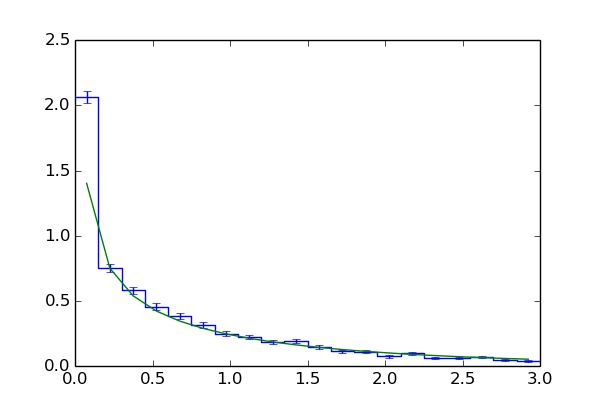
two-dimensional histograms. In line 38 we plot the (density) histogram and in
line 39 we superimpose a
are the boundaries of the corresponding bin. To
estimate the PDF for we have to divide each data value by
the bin width. This is done in line 37, using myFitter’s
densityHistogram() function. This function works on one and
two-dimensional histograms. In line 38 we plot the (density) histogram and in
line 39 we superimpose a  distribution with one degree of freedom
(using functions from scipy.stats).
distribution with one degree of freedom
(using functions from scipy.stats).
Computing p-values
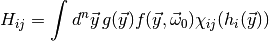
Although ToySimulator can be used as a generator for toy observables, its real purpose is the computation of expectation values of arbitrary functions on observable space. Let
be such a function and a point in parameter
space. Its expectation value of  at
at  is
is
(1)![E_{\vec\omega_0}[g] = \int d^n\vec y\, g(\vec y)f(\vec y,\vec\omega_0)
\eqsep.](_images/math/ed4450282b470773fef6545604064f5a4f3bdb96.png)
To compute this integral ToySimulator uses the VEGAS algorithm for adaptive Monte Carlo integration implemented in the Python module vegas together with a suitable re-parametrisation of the integrand. Since such integrations can take a long time ToySimulator also supports parallelisation.
As discussed in Statistical inference the (plug-in) p-value of a
likelihood ratio test is the probability that the value of
a randomly generated set of toy observables is larger than the observed
value. It is given by the integral (1) with
(2)
where  is the Heavyside step function and is the
observed data. The LRTIntegrand class implements this
function. To instantiate it, you need two Fitter objects
which fit the full model and the model representing the null hypothesis,
respectively, and the value of . Here is an
example using the model from previous examples (see also
toy_example_2.py):
is the Heavyside step function and is the
observed data. The LRTIntegrand class implements this
function. To instantiate it, you need two Fitter objects
which fit the full model and the model representing the null hypothesis,
respectively, and the value of . Here is an
example using the model from previous examples (see also
toy_example_2.py):
import numpy as np
import matplotlib.pyplot as plt
import scipy.stats as stats

model0 = MyModel()
model0.fix({'p1' : 1.25})
fitter0 = mf.Fitter(model0, tries=1)
fitter0.sample(2000)
fit0 = fitter0.fit()

model1 = MyModel()
fitter1 = mf.Fitter(model1, tries=1)
fitter1.sample(2000)
fit1 = fitter1.fit()

dchisq = fit0.minChiSquare - fit1.minChiSquare
lrt = mf.LRTIntegrand(fitter0, fitter1, dchisq, nested=True)
The object lrt is callable and takes a dict representing the point
in observable space as argument. It returns a numpy array of two
elements. The first element is the value of  from
(2). The second is the value of and can
be used for histogramming (see below). If the
third argument in the constructor is omitted the first element of the array
returned by lrt is always 1. LRTIntegrand objects
count the number of failed evaluations where one of the minimisations did not
converge or could not find a feasible solution. This number is stored in
LRTIntegrand.nfail. The total number of
evaluations is stored in LRTIntegrand.nshots. In a good simulation the fraction of failed evaluations
should be small, so this information is important to assess the reliability of
your results. The nested=True argument indicates that fitter0.model and
fitter1.model have the same parameters, so that the best-fit parameters for
fitter0.model can be used as a starting point for the fit of
fitter1.model. LRTIntegrand uses this trick to improve
the numerical stability.
from
(2). The second is the value of and can
be used for histogramming (see below). If the
third argument in the constructor is omitted the first element of the array
returned by lrt is always 1. LRTIntegrand objects
count the number of failed evaluations where one of the minimisations did not
converge or could not find a feasible solution. This number is stored in
LRTIntegrand.nfail. The total number of
evaluations is stored in LRTIntegrand.nshots. In a good simulation the fraction of failed evaluations
should be small, so this information is important to assess the reliability of
your results. The nested=True argument indicates that fitter0.model and
fitter1.model have the same parameters, so that the best-fit parameters for
fitter0.model can be used as a starting point for the fit of
fitter1.model. LRTIntegrand uses this trick to improve
the numerical stability.
With the assignments above the p-value can be computed as follows (see also toy_example_2.py):
1 2 3 4 5 6 7 8 | sim = mf.ToySimulator(model0, fit0.bestFitParameters,
parallel={'njobs' : 2,
'runner' : mf.LocalRunner})
result = sim(lrt, nitn=5, neval=2000, drop=1, log=sys.stdout)
print
print 'p-value: '+str(mf.GVar(result[0]))
print 'asymptotic p-value: {0:f}'.format(mf.pvalueFromChisq(dchisq, 1))
|
In line 1 we construct the ToySimulator object. The first
two arguments mean that  is the PDF of model0 and that
are the maximum likelihood estimates of the parameters
found in our earlier fit of model0. This means
we are going to compute the plug-in p-value.
is the PDF of model0 and that
are the maximum likelihood estimates of the parameters
found in our earlier fit of model0. This means
we are going to compute the plug-in p-value.
The parallel keyword to the constructor (line 2) enables parallelisation and works the same way as for Profiler1D or Profiler2D (see Parallelisation). In line 4 we perform the integration by calling the object sim. The first argument is the integrand function. Since we want the p-value we use the LRTIntegrand object constructed earlier.The VEGAS integration proceeds in several iterations, and after each iteration the results from all iterations are used to adapt the sampling density to the integrand. (Our integrand function actually returns an array with two values, but the adaptation is always driven by the first element of the array.) The final result is the weighted average of the results from all iterations. The allowed keyword arguments to ToySimulator.__call__() are the same as for the ToySimulator constructor and can be used to override the settings made there. The argument nitn=5 means that we run 5 iterations, and neval=2000 limits the number of integrand evaluations in each iteration to 2000. For difficult integrands the estimates from the first few iterations can be rather poor and their errors can be vastly underestimated. It is therefore usually better to exclude the results of the first few iterations from the weighted average. With drop=1 we instruct sim to exclude the result of the first iteration. The log=sys.stdout argument means that information about the iterations will be written to sys.stdout. Only information about the first integrand (i.e. the first element of the array returned by lrt) is written. The output will be something like
itn                  integral               wgt average  chi2/dof     Q
-----------------------------------------------------------------------
  1                0.0924(88)                0.0924(88)
  1                0.0912(60)                0.0912(60)
  2                0.0854(46)                0.0876(37)       0.6   44%
  3                0.0965(89)                0.0889(34)       0.7   48%
  4                0.0910(33)                0.0900(24)       0.6   64%
The second column shows the estimates of the integral from the individual
iterations. The number in brackets is the error on the last digit. Thus,
 means
means  . The third column shows the
weighted average of the results from all iterations (except the ones that were
dropped) and the first column shows the number of iterations included in the
weighted average. The numbers in the fourth and fifth columns are useful to
assess the compatibility of the results included in the weighted average. For a
reliable integration result the number in the fourth column should be of order 1
and the number in the fifth column should not be too small—say, above 5%. It
is worth mentioning that, at least in this example, the VEGAS adaptation actually
doesn’t reduce the integration error in a noticable way: the errors of the
results in the second column do not decrease significantly as the integration
progresses.
. The third column shows the
weighted average of the results from all iterations (except the ones that were
dropped) and the first column shows the number of iterations included in the
weighted average. The numbers in the fourth and fifth columns are useful to
assess the compatibility of the results included in the weighted average. For a
reliable integration result the number in the fourth column should be of order 1
and the number in the fifth column should not be too small—say, above 5%. It
is worth mentioning that, at least in this example, the VEGAS adaptation actually
doesn’t reduce the integration error in a noticable way: the errors of the
results in the second column do not decrease significantly as the integration
progresses.
In myFitter the result of a VEGAS integration is represented by instances of the IntegrationResult class. IntegrationResult objects hold the results and errors of the individual iterations as well as their weighted average, chi-square (which has nothing to do with the chi-square function of your model), Q-value, and the error of the weighted average. Since our integrand function returns an array of two values the return value of sim in line 4 is an array of two IntegrationResult objects. Since we only want the p-value we are only interested in the first element of this array. In line 7 we print the p-value and its numerical error by converting result[0] first to a GVar object and then to a string. In line 8 we print the asymptotic approximation of the p-value. The output is
p-value:            0.0900(24)
asymptotic p-value: 0.117566
The difference between the numerical result and the asymptotic approximation is about 11 times larger than the numerical error, which shows that the asymptotic approximation is not exact for this model.
The myFitter method
So far we have only computed relatively large p-values with toy simulations. As mentioned at the beginning of this chapter, “naive” toy simulations become very inefficient for small p-values, and the unique feature of myFitter is an advanced method for the numerical computation of very small p-values. This is achived by a clever re-parametrisation of the (p-value) integrand which uses information not only from the model describing the null hypothesis (model0) but also from the full model (model1).
To illustrate this feature let us now choose the null hyptothesis p1 = 1.1
(with all other parameters treated as nuisance parameters). This hypothesis has
a value of 11.2 and an asymptotic p-value of  . A naive toy simulation would need more than
  integrand
evaluations to estimate such a small p-value with a relative 10% accuracy. The
following code estimates the p-value using the myFitter method (see also
toy_example_3.py):
integrand
evaluations to estimate such a small p-value with a relative 10% accuracy. The
following code estimates the p-value using the myFitter method (see also
toy_example_3.py):
1 2 3 4 5 6 7 8 9 10 11 12 13 14 15 16 17 18 19 20 21 22 23 24 | model0 = MyModel()
model0.fix({'p1' : 1.1})
fitter0 = mf.Fitter(model0, tries=1)
fitter0.sample(2000)
fit0 = fitter0.fit()
model1 = MyModel()
fitter1 = mf.Fitter(model1, tries=1)
fitter1.sample(2000)
fit1 = fitter1.fit()
dchisq = fit0.minChiSquare - fit1.minChiSquare
lrt = mf.LRTIntegrand(fitter0, fitter1, dchisq, nested=True)
sim = mf.ToySimulator(model0, fit0.bestFitParameters,
model1=model1,
dchisq=dchisq,
parallel={'njobs' : 2,
'runner' : mf.LocalRunner})
result = sim(lrt, nitn=5, neval=10000, drop=1, log=sys.stdout)
print
print 'p-value: {0:s}'.format(str(mf.GVar(result[0])))
print 'asymptotic p-value: {0:f}'.format(mf.pvalueFromChisq(dchisq, 1))
|
Apart from changing the value of p1 and increasing the number of evaluations per iteration (neval) a little the only difference to the previous example is the addition of the model1 and dchisq keyword arguments in lines 16 and 17. With this extra information ToySimulator constructs a smart sampling density which is taylored for the p-value integrand constructed in line 13. The output of the program is
itn                  integral               wgt average  chi2/dof     Q
-----------------------------------------------------------------------
  1              0.000468(17)              0.000468(17)
  1              0.000471(14)              0.000471(14)
  2              0.000488(21)              0.000476(11)       0.5   49%
  3              0.000505(11)             0.0004905(81)       1.9   15%
  4              0.000483(10)             0.0004875(63)       1.4   24%

p-value:            0.0004875(63)
asymptotic p-value: 0.000808
Note that the first iteration with  evaluations already estimates
the p-value with a relative accuracy of less than 10%. With the naive method
from Generating toy observables this would require evaluations—a
factor improvement in efficiency. The final relative accuracy of
1.3%, achieved with the myFitter method after 50 000 evaluations, would require
evaluations already estimates
the p-value with a relative accuracy of less than 10%. With the naive method
from Generating toy observables this would require evaluations—a
factor improvement in efficiency. The final relative accuracy of
1.3%, achieved with the myFitter method after 50 000 evaluations, would require
 evaluations with the naive method. That’s a factor
 improvement in efficiency! Also note that the numerical
result for the p-value differs from the asymptotic approximation by almost a
factor of 2.
improvement in efficiency! Also note that the numerical
result for the p-value differs from the asymptotic approximation by almost a
factor of 2.
Filling histograms
In our initial example we used a toy simulation to compute the p-value and fill a histogram at the same time. For the advanced integration methods discussed in Computing p-values and The myFitter method this is no longer possible. You can, however, use the ToySimulator.fill() method to fill one or more histograms without programming the loop over toy observables yourself. This has the advantage that you automatically get errors estimates for the bin heights. More importantly, you can let ToySimulator parallelise the task of filling histograms for you (just like it automatically parallelises the VEGAS integration).
To understand how fill() works let us first
formalise the problem a little. Assume you want to compute the expectation value
(1) for some function on observable space. At the same time you
have functions  on observable space which you want to histogram,
i.e. you are also interested in the integrals
on observable space which you want to histogram,
i.e. you are also interested in the integrals
(3)
where  is an indicator function which is 1 if
  is
in the
is
in the  -th bin of the
  -th histogram and 0 otherwise. The
notation also applies to two-dimensional histograms, in which case the functions
must return a two-component vector. The example from
Toy simulations corresponds to the case
-th histogram and 0 otherwise. The
notation also applies to two-dimensional histograms, in which case the functions
must return a two-component vector. The example from
Toy simulations corresponds to the case
(4)
To compute ![E_{\vec\omega_0}[g]](_images/math/a903239fc62f0f1859651116c719332a841cf460.png) and fill all the histograms in one
simulation you just have to define a Python function—call it gh—which
takes a dict describing the point in observable space as
argument and which returns a list (or numpy array) holding the values of
,
and fill all the histograms in one
simulation you just have to define a Python function—call it gh—which
takes a dict describing the point in observable space as
argument and which returns a list (or numpy array) holding the values of
,  etc. (the zeroth element being
). For the case (4) we can just use an
LRTIntegrand object for gh. If we omit the
third argument (dchisq) in the constructor the first element of the
returned array will always be 1.
etc. (the zeroth element being
). For the case (4) we can just use an
LRTIntegrand object for gh. If we omit the
third argument (dchisq) in the constructor the first element of the
returned array will always be 1.
The following code uses fill() to compute the same histogram as in Toy simulations (see also toy_example_4.py):
1 2 3 4 5 6 7 8 9 10 11 12 13 14 15 16 17 18 19 20 21 22 23 24 | model0 = MyModel()
model0.fix({'p1' : 1.25})
fitter0 = mf.Fitter(model0, tries=1)
fitter0.sample(2000)
fit0 = fitter0.fit()
model1 = MyModel()
fitter1 = mf.Fitter(model1, tries=1)
fitter1.sample(2000)
dchisqhist = mf.Histogram1D(xbins=np.linspace(0.0, 3.0, 21))
sim = mf.ToySimulator(model0, fit0.bestFitParameters,
parallel={'njobs' : 2,
'runner' : mf.LocalRunner,
'log' : sys.stdout})
gh = mf.LRTIntegrand(fitter0, fitter1, nested=True)
sim.fill(gh, 10000, (1, dchisqhist))
dchisqhist = mf.densityHistogram(dchisqhist)
dchisqhist.plot(drawstyle='steps', color='b')
dchisqhist.errorbars(color='b')
plt.plot(dchisqhist.xvals, [stats.chi2.pdf(x, 1) for x in dchisqhist.xvals])
plt.show()
|
Lines 1 to 15 are mostly the same as in previous examples. Note that we have added 'log' : sys.stdout to the dict assigned to the parallel keyword in line 15. This causes ToySimulator to print information about the running jobs to stdout. In line 16 we create a LRTIntegrand object and assign it to gh. Note the omission of the dchisq argument in the constructor. This means the first element of the array returned by gh is always 1.
In line 18 we call fill to carry out the
simulation and fill the histogram. The first argument is the integrand function
gh. The second argument is the (maximal) number of evaluations. The third
argument (1, dchisqhist) instructs fill
to use element 1 of the list returned by gh to fill the histogram
dchisqhist. This element holds the value. You can fill
more than one histogram by adding more tuples to the argument list of
fill. The second element of each tuple must
be a Histogram1D or Histogram2D
object. If it is a Histogram2D object the first element
must be a tuple of two integers which specify the positions of the two variables
to be histogrammed in the list returned by gh. Alternatively, the first
element of the tuple can be a callable object. See the reference of
fill for details.
After line 18 the data values of dchisqhist are GVar
objects which hold the estimates and errors of the integrals (3). The
return value of fill is a
GVar object holding the estimate and error of the integral
(1). In our example we do not need this estimate (it is 1 with an error of
0 since our function is identical to 1), so we discard it. In lines
21 and 22 we plot the histogram with errorbars. Note that you don’t need the
convert keyword to turn GVar objects into ordinary
numbers. Histogram1D and Histogram2D
know what to do with data values of type GVar.