Statistical inference
The procedure of drawing conclusions about model parameters from randomly distributed data is known as statistical inference. This section explains the mathematical theory behind statistical inference. If you are already familiar with this subject feel free to skip to the next section.
General case
For a statistician a model is simply a probability density function (PDF)
 , which describes the (joint) distribution of a set of observables
 in the sample space
  and
depends on some parameters
and
depends on some parameters  . The parameter space
 can be any (discrete or continuous) set and can be any
function of
can be any (discrete or continuous) set and can be any
function of  and
and  with
with
(1)
for all . Statistical inference can help us answer
the following questions:
- Which choice of the parameters is most compatible with some observed
data
 ?
? - Based on the observed data
 , which parts of the parameter
space can be ruled out (at which confidence level)?
, which parts of the parameter
space can be ruled out (at which confidence level)?
Let us begin with the first question. What we need is a function
 which assigns to each observable vector
an estimate of the model parameters. Such a function is called an
estimator. There are different ways to define an estimator, but the most
popular choice (and the one that myFitter supports) is the
maximum likelihood estimator defined by
which assigns to each observable vector
an estimate of the model parameters. Such a function is called an
estimator. There are different ways to define an estimator, but the most
popular choice (and the one that myFitter supports) is the
maximum likelihood estimator defined by
In other words, for a given observation the maximum likelihood
estimate of the parameters are those parameters which maximise  . When we keep the observables fixed and regard as a function
of the parameters we call it the likelihood function. Finding the maximum of
the likelihood function is commonly referred to as fitting the model
to the data . It usually requires numerical optimisation
techniques.
. When we keep the observables fixed and regard as a function
of the parameters we call it the likelihood function. Finding the maximum of
the likelihood function is commonly referred to as fitting the model
to the data . It usually requires numerical optimisation
techniques.
The second question is answered (in frequentist statistics) by performing a
hypothesis test. Let’s say we want know if the model is realised with
parameters from some subset  . We call this the
null hypothesis. To test this hypothesis we have to define some function
. We call this the
null hypothesis. To test this hypothesis we have to define some function
 , called test statistic, which quantifies the disagreement of
the observation with the null hypothesis. The phrase
“quantifying the disagreement” is meant in the rather vague sense that
should be large when looks like it was not
drawn from a distribution with parameters in
, called test statistic, which quantifies the disagreement of
the observation with the null hypothesis. The phrase
“quantifying the disagreement” is meant in the rather vague sense that
should be large when looks like it was not
drawn from a distribution with parameters in  . In principle any
function on
. In principle any
function on  can be used as a test statistic, but of course
some are less useful than others. The most popular choice (and the one
myFitter is designed for) is
can be used as a test statistic, but of course
some are less useful than others. The most popular choice (and the one
myFitter is designed for) is
For this choice of  , the test is called a likelihood ratio test.
With a slight abuse of notation, we define
, the test is called a likelihood ratio test.
With a slight abuse of notation, we define
(2)
Then we may write
(3)
Clearly large values of  indicate that the null hypothesis
is unlikely, but at which value should we reject it? To determine that we have to
compute another quantity called the p-value
indicate that the null hypothesis
is unlikely, but at which value should we reject it? To determine that we have to
compute another quantity called the p-value
(4)
where  is the Heavyside step function. Note that the integral is
simply the probability that for some random vector
is the Heavyside step function. Note that the integral is
simply the probability that for some random vector  of toy
observables drawn from the distribution
of toy
observables drawn from the distribution  the test
statistic
the test
statistic  is larger than the observed value
 . The meaning of the p-value is the following: if
the null hypothesis is true and we reject it for values of
larger than the observed value the probability
for wrongly rejecting the null hypothesis is at most
. The meaning of the p-value is the following: if
the null hypothesis is true and we reject it for values of
larger than the observed value the probability
for wrongly rejecting the null hypothesis is at most  . Thus, the smaller the p-value, the more confident we can be in rejecting
the null hypothesis. The complementary probability
. Thus, the smaller the p-value, the more confident we can be in rejecting
the null hypothesis. The complementary probability  is therefore called the confidence level at which we may reject the null
hypothesis , based on the observation .
is therefore called the confidence level at which we may reject the null
hypothesis , based on the observation .
Instead of specifying the p-value directly people often give the Z-value (or number of ‘standard deviations‘ or ‘sigmas‘) which is related to the p-value by
where ‘ ‘ denotes the error function. The relation is chosen in such
a way that the integral of a normal distribution from
‘ denotes the error function. The relation is chosen in such
a way that the integral of a normal distribution from  to
to  is the confidence level
  . So, if someone tells you that they have
discovered something at
. So, if someone tells you that they have
discovered something at  they have (usually) done a likelihood
ratio test and rejected the “no signal” hypothesis at a confidence level
corresponding to
they have (usually) done a likelihood
ratio test and rejected the “no signal” hypothesis at a confidence level
corresponding to  .
.
Linear regression models and Wilks’ theorem
Evaluating the right-hand side of (4) exactly for a realistic model can be extremely challenging. However, for a specific class of models called linear regression models we can evaluate (4) analytically. The good news is that most models can be approximated by linear regression models and that this approximation is often sufficient for the purpose of estimating the p-value. A concrete formulation of this statement is given by a theorem by Wilks, which we shall discuss shortly. The myFitter package was originally written to handle problems where Wilks’ theorem is not applicable, but of course the framework can also be used in cases where Wilks’ theorem applies.
In a linear regression model the parameter space  is a
is a
 -dimensional real vector space and the PDF is a
(multi-dimensional) normal distribution with a fixed
(i.e. parameter-independent) covariance matrix
-dimensional real vector space and the PDF is a
(multi-dimensional) normal distribution with a fixed
(i.e. parameter-independent) covariance matrix  centered on an
observable-vector
centered on an
observable-vector  which is an affine-linear function
of the parameters :
which is an affine-linear function
of the parameters :
(5)![f(\vec x,\vec\omega) &= \mathcal{N}(\vec\mu(\vec\omega), \Sigma)(\vec x)
\propto \exp[-\tfrac12(\vec x-\vec\mu(\vec\omega))^\trans \Sigma^{-1}
(\vec x-\vec\mu(\vec\omega))]
\eqsep,\\
\vec\mu(\vec\omega) &= A\vec\omega + \vec b
\eqsep,](_images/math/c615d9870c3fc73cf6983b83826bdf449448f79d.png)
where is a symmetric, positive definite matrix,  is a
non-singular (
is a
non-singular ( )-matrix and
  is a
is a
 -dimensional real vector. Now assume that the parameter space
under the null hypothesis is a
-dimensional real vector. Now assume that the parameter space
under the null hypothesis is a  -dimensional affine
sub-space of (i.e. a linear sub-space with a constant shift).
In this case the formula (4) for the p-value becomes
-dimensional affine
sub-space of (i.e. a linear sub-space with a constant shift).
In this case the formula (4) for the p-value becomes
(6)
where  is the normalised upper incomplete Gamma function which can be
found in any decent special functions library. Note that, for a linear regession
model, the p-value only depends on the dimension of the affine sub-space
but not on its position within the larger space .
is the normalised upper incomplete Gamma function which can be
found in any decent special functions library. Note that, for a linear regession
model, the p-value only depends on the dimension of the affine sub-space
but not on its position within the larger space .
The models we encounter in global fits are usually not linear regession models.
They typically belong to a class of models known as non-linear regression
models. The PDF of a non-linear regression model still has the form
(5) with a fixed covariance matrix , but the
means  may depend on the parameters in an
arbitrary way. Furthermore, the parameter spaces and
don’t have to be vector spaces but can be arbitrary smooth
manifolds. The means of a non-linear regression model are
usually the theory predictions for the observables and have a known functional
dependence on the parameters of the theory. The information
about experimental uncertainties (and correlations) is encoded in the covariance
matrix .
may depend on the parameters in an
arbitrary way. Furthermore, the parameter spaces and
don’t have to be vector spaces but can be arbitrary smooth
manifolds. The means of a non-linear regression model are
usually the theory predictions for the observables and have a known functional
dependence on the parameters of the theory. The information
about experimental uncertainties (and correlations) is encoded in the covariance
matrix .
Since any smooth non-linear function can be locally approximated by a linear
function it seems plausible that (6) can still hold approximately even
for non-linear regression models. This is essentially the content of Wilks’
theorem. It states that, for a general model (not only non-linear regression
models) which satisfies certain regularity conditions, (6) holds
asymptotically in the limit of an infinite number of independent
observations. The parameter spaces and in the
general case can be smooth manifolds with dimensions and
, respectively. Note, however, that for Wilks’ theorem to hold
must still be a subset of .
Plug-in p-values and the myFitter method
In practice we cannot make an arbitrarily large number of independent
observations. Thus (6) is only an approximation whose quality depends on
the amount of collected data and the model under consideration. To test the
quality of the approximation (6) for a specific model one must evaluate
or at least approximate (4) by other means, e.g. numerically. Such
computations are called toy simulations, and their computational cost can be
immense. Note that the evaluation of (and thus of the
integrand in (4)) requires a numerical optimisation. And then the
integral in (4) still needs to be maximised over  .
.
In most cases the integral is reasonably close to its maxiumum value when
is set to its maximum likelihood estimate for the
observed data and the parameter space :

Thus, the plug-in p-value
is often a good approximation to the real p-value.
The standard numerical approach to computing the remaining integral is to
generate a large number of toy observations  distributed according to
  and then determine the fraction of toy observations where
 . If the p-value is small
this method can become very inefficient. The efficiency can be significantly
improved by importance sampling methods, i.e. by drawing toy observations
from some other (suitably constructed) sampling density which avoids the region
with
. If the p-value is small
this method can become very inefficient. The efficiency can be significantly
improved by importance sampling methods, i.e. by drawing toy observations
from some other (suitably constructed) sampling density which avoids the region
with 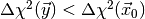 . This method lies at
the heart of the myFitter package.
. This method lies at
the heart of the myFitter package.
Gaussian and systematic errors
As mentioned above the most common type of model we deal with in global fits are
non-linear regression models where the means
represent theoretical predictions for the
observables and the information about experimental uncertainties is encoded in
the covariance matrix . If the value of an observable is given as
 in a scientific text this usually implies that the observable
has a Gaussian distribution with a standard deviation of 0.5. Measurements
from different experiments are usually uncorrelated. Thus the covariance matrix
for independent observables is
in a scientific text this usually implies that the observable
has a Gaussian distribution with a standard deviation of 0.5. Measurements
from different experiments are usually uncorrelated. Thus the covariance matrix
for independent observables is
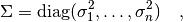
where the  are the errors of the individual measurements. If
several quantities are measured in the same experiment they can be correlated.
Information about the correlations is usually presented in the form of a
correlation matrix
are the errors of the individual measurements. If
several quantities are measured in the same experiment they can be correlated.
Information about the correlations is usually presented in the form of a
correlation matrix  . The correlation matrix is always symmetric
and its diagonal entries are 1. (Thus it is common to only show the lower or
upper triangle of in a publication.) The elements
. The correlation matrix is always symmetric
and its diagonal entries are 1. (Thus it is common to only show the lower or
upper triangle of in a publication.) The elements  of are called correlation coefficients. For observables
with errors and correlation coefficients
the covariance matrix is given by
of are called correlation coefficients. For observables
with errors and correlation coefficients
the covariance matrix is given by

In some cases the error of an observable is broken up into a statistical and a
systematic component. Typical notations are  or simply
  with an indication which
component is the systematic one given in the text. Sometimes the systematic
error is asymmetric and denoted as
with an indication which
component is the systematic one given in the text. Sometimes the systematic
error is asymmetric and denoted as  .
.
What are we supposed to do with this extra information? This depends largely on
the context, i.e. on the nature of the systematic uncertainties being
quoted. For example, the theoretical prediction of an observable  (or
its extraction from raw experimental data) might require knowledge of some other
quantity
(or
its extraction from raw experimental data) might require knowledge of some other
quantity  which has been measured elsewhere with some Gaussian
uncertainty. In this case one also speaks of a parametric uncertainty. If you
know the dependence of on it is best to treat
as a parameter of your model, add an observable which represents
the measurement of (i.e. with a Gaussian distribution centered
on and an appropriate standard deviation), and use only the
statistical error to model the distribution of . In particular, this is
the only (correct) way in which you can combine with other observables
that depend on the same parameter . In this case the parameter
is called a nuisance parameter, since we are not interested in
its value but need it to extract values for the parameters we are interested in.
which has been measured elsewhere with some Gaussian
uncertainty. In this case one also speaks of a parametric uncertainty. If you
know the dependence of on it is best to treat
as a parameter of your model, add an observable which represents
the measurement of (i.e. with a Gaussian distribution centered
on and an appropriate standard deviation), and use only the
statistical error to model the distribution of . In particular, this is
the only (correct) way in which you can combine with other observables
that depend on the same parameter . In this case the parameter
is called a nuisance parameter, since we are not interested in
its value but need it to extract values for the parameters we are interested in.
If you don’t know the dependence of on but you are
sure that the systematic uncertainty for given in a paper is (mainly)
parametric due to and that does not affect any
other observables in your fit you can combine the statistical and systematic
error in quadrature. This means you assume a Gaussian distribution for
with standard deviation  , where
  is the
statistical and
is the
statistical and  the systematic error (which should be
symmetric in this case). This procedure is also correct if the systematic error
is the combined parametric uncertainty due to several parameters, as long as
none of these parameters affect any other observables in your fit.
the systematic error (which should be
symmetric in this case). This procedure is also correct if the systematic error
is the combined parametric uncertainty due to several parameters, as long as
none of these parameters affect any other observables in your fit.
So far in our discussion we have assumed that the nuisance parameter(s) can be measured and have a Gaussian
distribution. This is not always the case. If, for example, the theoretical
prediction for an observable is an approximation there will be a constant offset
between the theory prediction and the measured value. This offset does not
average out when the experiment is repeated many times, and it cannot be
measured separately either. At best we can find some sort of upper bound on the
size of this offset. The extraction of an observable from the raw data may also
depend on parameters which can only be bounded but not measured. In this case
the offset between the theory prediction and the mean of the measured quantity
should be treated as an additional model parameter whose values are restricted
to a finite range. Assume that the systematic error of is given as
 with
with  . Let
. Let
 be the theory prediction for . The
mean
be the theory prediction for . The
mean  of the observable then depends on an additional
nuisance parameter
of the observable then depends on an additional
nuisance parameter  which takes values in the interval
![[-\delta_-,+\delta_+]](_images/math/8f9cc14feb9c81a1e6fc499628c564365ba1b521.png) :
:
![\mu(\vec\omega,\delta) = \mu_\text{th}(\vec\omega) - \delta
\eqsep\text{with}\eqsep\delta\in[-\delta_-,+\delta_+]
\eqsep.](_images/math/36d7f3335de29fe8553095497e41a124c8dd11cb.png)
Note that the formula above holds for systematic uncertainties associated with
the measurement of . If the theory prediction for an observable
is quoted with a systematic error the correct
range for is ![[-\delta_+,+\delta_-]](_images/math/00514eea4c3385f9712de2d809c7115e8a32ae31.png) .
.