The Model class
Before you can do fits with myFitter you have to define the model you want to
fit. All models in myFitter are represented by classes derived from the
Model class. Each Model instance has
four dict attributes which, together, fully specify the parameter space
 , the sample space
  , the PDF
  and the
observed data
and the
observed data  (see Statistical inference for definitions). The
dictionaries are called par, con,
csc, and obs. When you define your own
model class it is your responsibility to fill these dictionaries with the
appropriate data. This is most conveniently done in the
__init__() method. The keys of the dictionaries can
be arbitrarily chosen strings. Most of the time you will not modify the
dictionaries directly but via various Model.add... methods which we will
discuss shortly. However, to understand the arguments to some of these methods
it is good to know what the par, con,
csc, and obs dicts contain.
(see Statistical inference for definitions). The
dictionaries are called par, con,
csc, and obs. When you define your own
model class it is your responsibility to fill these dictionaries with the
appropriate data. This is most conveniently done in the
__init__() method. The keys of the dictionaries can
be arbitrarily chosen strings. Most of the time you will not modify the
dictionaries directly but via various Model.add... methods which we will
discuss shortly. However, to understand the arguments to some of these methods
it is good to know what the par, con,
csc, and obs dicts contain.
- par
- holds the parameters of the model. The values must be instances of Parameter. Amongst other things, Parameter instances hold information about upper and lower bounds of the associated parameter.
- con
- holds constraints (other than upper or lower bounds on individual parameters) on the model’s parameter space. Non-linear constraints such as x*y == 1 or x*y < 1 can be imposed through this dictionary. The values must be instances of Constraint.
- csc
- holds the model’s chi-square contributions (see below). Values must be instances of ChiSquareContribution.
- obs
- holds the components of the vector
In addition there is the nuisanceCSCs member which is a set holding the names of the CSCs associated with nuisance parameters. Its purpose will be explained in Manipulating Model objects.
Chi-square contributions
As explained in Statistical inference, all information about a statistical model is contained in the probability density function

where is the model’s parameter space and  the space of observables or sample space. The same information is contained
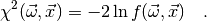
in the chi-square function which is defined (in myFitter) as
the space of observables or sample space. The same information is contained
in the chi-square function which is defined (in myFitter) as
In some cases, e.g. if the observables  were measured in different
experiments, the function is a product of individual factors
were measured in different
experiments, the function is a product of individual factors
 :
:
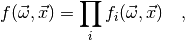
where each factor only depends on a subset of the observables
 . In this case the chi-square function is

The terms  are called chi-square contributions (CSCs) in
myFitter.
are called chi-square contributions (CSCs) in
myFitter.
CSCs are represented by instances of classes derived from ChiSquareContribution. You can implement your own CSCs by deriving from this class. However, the the most common types of CSCs are Gaussian CSCs with fixed errors and correlation matrix. These CSCs are already implemented by the GaussianCSC and CorrelatedGaussianCSC classes.
Dependent quantities and observables
The shape of a CSC is usually characterised by one or more
quantities which may depend on the model parameters in an arbitrary way. For
example, a Gaussian CSC is centred on a mean value  which can be an arbitrary function of the model parameters. Quantities like
are called dependent quantities in myFitter. In particular the
model parameters themselves are also dependent quantities. Each dependent
quantity in a model has a uniqe name which is a string you are free to choose
when you define the model. Values for dependent quantities are passed between
different myFitter functions by means of Python dicts whose keys are the
names of the dependent quantities.
which can be an arbitrary function of the model parameters. Quantities like
are called dependent quantities in myFitter. In particular the
model parameters themselves are also dependent quantities. Each dependent
quantity in a model has a uniqe name which is a string you are free to choose
when you define the model. Values for dependent quantities are passed between
different myFitter functions by means of Python dicts whose keys are the
names of the dependent quantities.
You specify the relationship between the model parameters and other dependent quantities by overriding the getDependentQuantities() method. It takes a dictionary with the parameters as argument and should return a dictionary which contains the parameters and any dependent quantities needed by the CSCs in your model.
Python dicts with strings as keys are also used to represent observable
vectors, i.e. elements of the sample space . This way each
component of the observable vector can be labelled by a
descriptive name you choose. You can (and typically will) use the same name for
an observable and a related dependent quantity since dependent quantities and
observables are never put in the same dictionary.
Deriving the model class
To see how all this works in detail let’s take a look at an example (see also mymodel.py):
1 2 3 4 5 6 7 8 9 10 11 12 13 14 15 16 17 18 19 20 21 22 23 24 25 26 27 28 29 30 31 32 | import myFitter as mf
class MyModel(mf.Model):
def __init__(self):
mf.Model.__init__(self)
self.addParameter('p1', default=1.0, bounds=(0.1, None))
self.addParameter('p2', default=1.0, scale=0.5)
self.addConstraint('p1 p2', '<', 1.0, scale=0.5)
self.addGaussianCSC('obs1', 2.05, 0.05, syst=(0.2, 0.1))
self.addCorrelatedGaussianCSC('obs234',
[('obs2', 0.8, 0.1),
('obs3', 2.3, 0.2),
('obs4', 0.3, 0.1)],
[('obs2', 'obs3', 0.2),
('obs3', 'obs4', -0.8)])
def getDependentQuantities(self, p):
q = mf.Model.getDependentQuantities(p)
p1 = q['p1']
p2 = q['p2']
q['p1 p2'] = p1*p2
q['obs1'] = p1**2 + p2**2
q['obs2'] = p2/p1
q['obs3'] = p1 + p2
q['obs4'] = p1 - p2
return q
|
In lines 6 and 7 we call the addParameter() method to add two parameters to the model. The strings 'p1' and 'p2' are the names of the parameters (i.e. the keys under which they are added to the par dict. With default=1.0 we state that the default value of parameter p1 is 1. If myFitter needs a value for the parameter p1 and you haven’t specified one it will take the default value. If no default value is given for a parameter myFitter assumes it is 0. With bounds=(0.1, None) we state that parameter p1 must be larger than 0.1, i.e. has a lower bound of 0 but no upper bound. With scale=0.5 we tell myFitter that “typical” values of p2 differ from the default value by something of the order of 0.5. This information is used by myFitter to generate random values for parameters and to improve the stability of numerical optimisations. If you do not specify a scale myFitter assumes a scale of 1. The keyword arguments to addParameter() are the same as the ones for constructor of the Parameter class.
In line 9 we call the addConstraint() method to impose a non-linear constraint on the model’s parameter space. Specifically, we require that p1 * p2 is smaller than 1. The first argument, 'p1 p2' is a dependent quantity which we must set to the product of p1 and p2 in getDependentQuantities(). The second and third argument state that this dependent quantity must be smaller than 1. The last argument tells myFitter that deviations of the quantity 'p1 p2' from its upper bound will typically be of the order of 0.5. Like the scale argument in addParameter() this information is used to improve numerical stability. The key under which this constraint is added to the con dict is generated from the first two arguments:
>>> MyModel().con.keys()
['p1 p2 <']
If you are not happy with this choice you can choose your own name with the name keyword argument. If you don’t want to introduce a separate dependent quantity for your constraint you can also pass a callable object as first argument to addConstraint(). This object will be called with the dict of dependent quantites (as returned by getDependentQuantities()) and should return the value of the constraint function. For example, the following code has the same effect as line 9:
self.addConstraint(lambda q: q['p1']*q['p2'], '<', 1.0,
                   scale=0.5, name='p1 p2 <')
Note that the name keyword must be specified in this case. Allowed values for the second argument are '<', '>', '=', and 'in'. The 'in' relation forces the constraint function to lie in a finite interval and can be used as follows:
self.addConstraint('p1 p2', 'in', (0.5, 2.0), scale=0.5)
In line 11 we call the addGaussianCSC() add a Gaussian
CSC to the model. Gaussian CSCs are represented by the
GaussianCSC class and can be added to a model with the
addGaussianCSC() method. The first argument 'obs1'
actually serves three purposes: it is the name which identifies the CSC within the model (i.e. the key under which it is added to the
csc dict), the name of the dependent quantity associated with the mean of the Gaussian, and the name of
the associated observable. If you want to use a different name for the dependent
quantity holding the mean of the Gaussian you can use the mean keyword
argument. See the documentation of addGaussianCSC()
for details. The second argument is the measured value of the
observable. (Thus, the obs dict will contain the key-value
pair 'obs1' : 2.05.) The third argument is the standard deviation of the
Gaussian. The syst keyword lets you specify the systematic uncertainty of the
observable. In the example we assign an asymmetric systematic uncertainty of
 . Thus the value observable 'obs1' would typically
be quoted as
. Thus the value observable 'obs1' would typically
be quoted as  in the literature. In accordance
with the discussion in Gaussian and systematic errors the specification of the
systematic error in line 11 adds a nuisance parameter to the model which is
subtracted from the mean of obs1 and which floats in the interval
in the literature. In accordance
with the discussion in Gaussian and systematic errors the specification of the
systematic error in line 11 adds a nuisance parameter to the model which is
subtracted from the mean of obs1 and which floats in the interval
![[-0.1, +0.2]](_images/math/b4b7537dc88e94a03a1e68e5044b349cf7e1ff9c.png) . The name of the nuisance parameter is constructed by
appending ' syst' (with a blank space) to the name of the observable. Thus,
our model now contains an additional parameter called 'obs1 syst' with an
appropriately chosen range. For symmetric systematic errors you can set the
syst keyword to a single number, e.g. syst=0.1.
. The name of the nuisance parameter is constructed by
appending ' syst' (with a blank space) to the name of the observable. Thus,
our model now contains an additional parameter called 'obs1 syst' with an
appropriately chosen range. For symmetric systematic errors you can set the
syst keyword to a single number, e.g. syst=0.1.
Line 12 introduces three correlated observables to the model. Since the PDF for correlated observables does not factorise we have to add a CSC which describes all three observables at once. The class CorrelatedGaussianCSC is made for this purpose and instances can be added to the model with the addCorrelatedGaussianCSC() method. The first argument is the name of the CSC (i.e. the key under which it is added to the csc dict). The second argument is a list of tuples which describes the observables, their measured values and standard deviations. In the example we define an observable with name 'obs2', measured value 0.8, and standard deviation 0.1, another observable 'obs3' with measured value 2.3 and standard deviation 0.2, etc. As for addGaussianCSC() the strings 'obs2', 'obs3', and 'obs4' are the keys under which the measured values are stored in the obs dict and also the names of the dependent quantities associated with the means. The means keyword argument of addCorrelatedGaussianCSC() lets you choose different names for the means. The third argument lists the correlation coefficients between the observables. The observables obs2 and obs3 have a correlation coefficient of 0.2 and the correlation between obs3 and obs4 is -0.8. Since no correlation between obs2 and obs4 is specified the corresponding correlation coefficient is set to zero.
The dependent quantities obs1, obs2, obs3, and obs4 (i.e. the means of the Gaussian observables) are all calculated in the getDependentQuantities() method. The argument p is a dict which specifies the values of the parameters. The keys of p must be a subset of the keys of the model’s par dict. In line 18 we call the method from the base class and assign the result to q. This should always be the first step when you define getDependentQuantities() in a derived class. The base class method performs the following operations:
- it makes an independent (deep) copy of the dictionary p,
- if any keys of the par dict are not present in p it substitutes them with their default values,
- if any parameters of the model have been fixed (e.g. with the fix() method) it sets these parameters to their fixed values.
As a result all parameters are guaranteed to be present in q and fixed parameters are guaranteed to have their fixed value. In lines 20 and 21 we read out the values of the parameters p1 and p2 from the dictionary q (not p). In lines 23 to 26 we compute the observables from the parameters p1 and p1 and add them to q under the keys 'obs1' to 'obs4'. Finally we return the dictionary q.
Gaussian nuisance parameters
As discussed in Gaussian and systematic errors your model may contain nuisance
parameters whose values have been determined with a
certain (Gaussian) uncertainty. It is straightforward to implement such nuisance
parameters with the functions discussed so far, but the
Model class also has a couple of methods specifically for
this purpose. Assume your model has a nuisance parameters  whose
measured value is
whose
measured value is  . Then you can simply add a parameter named
'lambda' to your model and an observable with the same name:
. Then you can simply add a parameter named
'lambda' to your model and an observable with the same name:
class MyModel(mf.Model):
    def __init__(self):
        ...
        self.addParameter('lambda', default=3.6, scale=0.4)
        self.addGaussianCSC('lambda', 3.6, 0.4)
        ...
Note that by choosing the same name for the parameter and the observable the dependent quantity which defines the mean of the Gaussian observable is identical to the parameter 'lambda' and does not need to be set explicitely in getDependentQuantities(). Of course you can set the default and scale attributes of the parameter 'lambda' to something else, but the central value and standard deviation of the measurement are usually a good choice.
The addGaussianNP() method of the Model class lets you do both of the definitions above in one line:
class MyModel(mf.Model):
    def __init__(self):
        ...
        self.addGaussianNP('lambda', 3.6, 0.4)
        ...
The arguments of the addGaussianNP() method are identical to the ones of addGaussianCSC(), but in addition to adding the observable it also adds a parameter with the same name and suitably chosen default and scale attributes. There is also a method called addCorrelatedGaussianNP() whose syntax is identical to addCorrelatedGaussianCSC() and which lets you add several correlated Gaussian nuisance parameters to your model.
Manipulating Model objects
The most common manipulations you will need to do on an existing model object is fixing the values of some of its parameters or (temporarily) removing certain constraints or CSCs. You can access the objects representing parameters, constraints, and CSCs directly through the model’s par, con, and csc attributes, respectively. In addition the Model has several methods which let you do these types of manipulations more easily.
To fix a parameter to a certain value you just have to set the value attribute of the Parameter object to the desired value. Setting the value attribute to None means that the parameter is not fixed. You can also use the fix() and release() methods of the Model class. The fix() method takes an arbitrary number of arguments which can be strings, lists of strings, or dicts. For dict arguments the keys should be parameter names, and the corresponding parameters will be fixed to the associated values. For string arguments or lists of strings the parameters will be fixed to their default values. The release() method takes an arbitrary number of strings or lists of strings as arguments and releases the corresponding parameters (i.e. sets their value attributes to None).
To temporarily remove a constraint or CSC from your model you don’t actually need to remove the objects from the con or csc dicts. Constraint and ChiSquareContribution objects have a boolean attribute called active which can be set to False to temporarily disable them.
The method deactivateConstraints() of the Model class can be used to disable several constraints at once. Like the release() method it takes an arbitrary number of arguments which can be strings or lists of strings identifying the constraints to de-activate. The method deactivateAllConstraints() can be used to de-activate all constraints of the model. The method deactivateOnlyConstraints() de-activates the specified constraints and activates all others. For activating specific constraints there is a matching set of methods called activateConstraints(), activateAllConstraints(), and activateOnlyConstraints(). Note that these methods only operate on the constraints listed in the con member of the Model object. Upper and lower bounds on individual parameters stored in the corresponding Parameter objects are not modified.
CSCs can be activated and de-activated by a matching set of methods called activateCSCs(), activateAllCSCs(), activateOnlyCSCs(), deactivateCSCs(), deactivateAllCSCs(), and deactivateOnlyCSCs(). If your model contains Gaussian nuisance parameters you typically want to keep the CSCs associated with the nuisance parameters active at all times. The deactivateAllCSCs() and activateAllCSCs() methods will therefore, by default, not change the state of any CSCs listed in the nuisanceCSCs member of your Model class. Likewise, activateOnlyCSCs() will not de-activate and deactivateOnlyCSCs() will not activate any of these CSCs. You can override this behaviour by setting the ignorenp keyword of these methods to False. The addGaussianNP() and addCorrelatedGaussianNP() methods will automatically add the names of the CSCs to the nuisanceCSCs member, but you can also modify this member directly.