Profiling the likelihood

If your model has more than two parameters the likelihood function can no longer be visualised in straightforward way. A common technique is to maximise the likelihood function with respect to all but one parameter and display the maximum value as a function of this parameter. Alternatively we can maximise with respect to all but two parameters and display the maximum value as a function of two variables (e.g. in a contour plot). This procedure is called profiling the likelihood, and the maximised functions are called (one or two-dimensional) profile likelihoods.

If you have implemented your model in a Model class and constructed a Fitter object which reliably finds the global minimum of the chi-square function the profile likelihood can be computed by a simple iteration. Continuing the previous example, we can profile the likelihood in the parameter 'p1' as follows (see also profile_example.py):

import numpy as np
import matplotlib.pyplot as plt

p1vals = np.linspace(1.0, 1.4, 41)
fitresults = []
for p1 in p1vals:
    fitter.clear()
    fitter.model.fix({'p1' : p1})
    fitter.sample(50)
    fitresults.append(fitter.fit(tries=3))
chisqvals = [r.minChiSquare for r in fitresults]

plt.plot(p1vals, chisqvals)
plt.show()

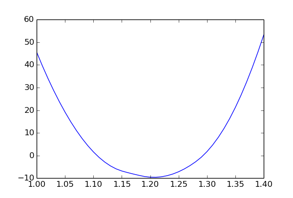
The plot shows the chi-square value as a function of p1 and minimised over the other two parameters (p2 and obs1 syst). The slight asymmetry is due to the non-linear constraint p1 * p2 < 1.

Note that, in the example above, we have to re-sample the parameter space for each value of p1. For difficult optimisation problems we need a large number of sample points to find the global minimum reliably, so this can take a lot of time. However, there is a simple trick which can improve the stability of profile likelihood computations significantly (and thus allow us to reduce the number of sample points). Assume that for p1 fixed to 1.3 the chi-square becomes minimal at p2=0.77. Then for p1 fixed to 1.31 the best-fit value of p2 will probably still be close to 0.77. Thus, to find the minimal chi-square for a given value of p1 we should use the best-fit values of the other parameters from adjacent p1 values as starting points for the local optimisation. We should still run a few minimisations from randomly chosen starting points since we also need to keep an eye out for other minima which may develop as p1 is varied, but if we use the information from adjacent points we can usually afford to be less thorough. The Profiler1D and Profiler2D classes use this trick to compute the profile likelihood on one and two-dimensional grids of points, respectively.

One-dimensional profiles

Continuing the example from Fitting the model, this is how you use a Profiler1D object to compute the profile likelihood in p1 (see also profile_example.py):

import numpy as np
import matplotlib.pyplot as plt

profiler = mf.Profiler1D('p1', fitter=fitter)
hist = mf.Histogram1D(xvals=np.linspace(1.0, 1.4, 41))
profiler.scan(hist, nsamples=50, tries=3)

hist.plot(convert=lambda r: r.minChiSquare)
plt.show()

In line 4 we create the Profiler1D object. The first argument identifies the variable in which the profile likelihood is computed. This can be the name of an arbitrary dependent quantity (not just a model parameter). The fitter keyword must be set to a properly initialised Fitter object which will then be used to perform global minimisations. In line 5 we define the grid on which the profile likelihood is computed by constructing a Histogram1D object. Histogram1D and Histogram2D are convenience classes defined in myFitter which let you store and visualise arbitrary data on one and two-dimensional grids, respectively. For each grid point they store a data value which can be an arbitrary Python object.

Line 6 performs the actual scan over p1. For each value of p1 the global minimisation is done with 50 sample points and 3 local minimisations. The nsamples and tries keywords can also be given to the constructor of Profiler1D. The Profiler1D.scan() method has several side effects. First of all, it sets the data values of the histogram hist to FitResult objects which represent the results of the minimisations for the individual grid points. It also uses the fitter object to re-sample the parameter space for each value of p1. Thus, any sample points stored in fitter before the call to scan() will be lost. If the variable specified in the constructor of Profiler1D is not a model parameter, scan() will also temporarily add a non-linear constraint to fitter.model which fixes the variable to the desired value. The name which scan() uses for this constraint is '__xscan__', so you should avoid using this name for one of your own constraints. Before scan() returns it removes the constraint.

The Histogram1D and Histogram2D classes both provide methods which allow you to visualise the data with matplotlib. Histogram1D provides the plot() method, which essentially mimicks the behaviour of matplotlib‘s plot function. Of course Histogram1D.plot() does not require arguments which specify the x and y values to plot, since it extracts those values from the histogram. However, if the data values stored in the histograms are not floats you have to provide a conversion function via the convert keyword which turns the data objects of your histogram into floats. In line 8 we set convert to an anonymous (lambda) function which returns the minChiSquare attribute of its argument. By default, Histogram1D.plot() draws the histogram to the “current” matplotlib axes object (as returned by matplotlib.pyplot.gca()), but you can specify a different axes object with the axes keyword. All other positional and keyword arguments are passed down to matplotlib.pyplot.plot(). For example, to make the step size of your grid of p1 values visible in the plot, try adding drawstyle='steps' to the argument list of Histogram1D.plot(). In line 9 we show the plot. The show function is explained in the matplotlib documentation.

A common application of profile likelihood functions is to find (approximate) confidence intervals for a parameter. In the asymptotic limit the p-value for the hypothesis that p1 has a certain value can be computed from the value by an analytic formula. The confidence interval of p1 at a given confidence level CL is then given by the region where the p-value is larger than 1-CL. Continuing the previous example, you can plot the p-value as follows (see also profile_example.py):

globalmin = min(globalmin, hist.min())
hist.plot(convert=lambda r: \
    mf.pvalueFromChisq(r.minChiSquare - globalmin.minChiSquare, 1))
sigmas = [mf.pvalueFromZvalue(z) for z in [1,2,3]]

plt.ylim((1e-4, 1.0))
plt.yscale('log')
plt.xlabel('p1')
plt.ylabel('p-value')

ax1 = plt.axes()
ax2 = ax1.twinx()
ax2.set_ylim(ax1.get_ylim())
ax2.set_yscale(ax1.get_yscale())
ax2.set_yticks(sigmas)
ax2.set_yticklabels([r'1 sigma', r'2 sigma', r'3 sigma'])
ax2.grid(True, axis='y')
plt.show()

The dashed horizontal lines indicate the p-values corresponding to one, two and three standard deviations (i.e. to Z-values of 1, 2, and 3). The relationship between p-values and Z-values was given earlier in this documentation. The associated confidence levels are (approximately) 68%, 95%, and 99.7%. The borders of the confidence intervals are the intersections of the blue curve with the dashed lines.

To compute the value we have to subtract the global minimum of the chi-square function from the chi-square values in hist. In principle the the value of globalmin computed earlier should be the global minimum of the chi-square function. However, in some cases the global minimisation fails and the profiler finds a point with a smaller chi-square value. The assignment in line 1 guarantees that globalmin is smaller than all the data values stored in hist. Note that we can use Python’s min function to compare FitResult objects since myFitter defines a total ordering for this class. The min() method of Histogram1D returns the smallest data value stored in the histogram.

In line 2 we plot the histogram with a conversion function that computes the p-value from the difference of chi-square values. It uses the myFitter function pvalueFromChisq() which uses the asymptotic formula to convert delta-chi-square values into p-values. The second argument is the number of degrees of freedom, which is 1 in this case since we are doing a one-dimenional scan. In line 4 we use the function pvalueFromZvalue() to compute the p-values corresponding to one, two and three standard deviations. To convert between p-values, Z-values and (delta) chi-square values myFitter defines the following functions: pvalueFromChisq(), chisqFromPvalue(), zvalueFromPvalue(), pvalueFromZvalue(), zvalueFromChisq(), and chisqFromZvalue().

The remaining code is specific to matplotlib library and explanations can be found in the documentation of matplotlib.

Two-dimensional profiles

Two-dimensional profile likelihoods can be computed in an analogous way using the Profiler2D class. Continuing the example from Fitting the model, this is how you can plot the 1, 2, and 3 sigma contours in the p1-p2-plane (see also profile_example.py):

profiler = mf.Profiler2D('p1', 'p2', fitter=fitter)
hist2d = mf.Histogram2D(xvals=np.linspace(1.0, 1.4, 31),
                      yvals=np.linspace(0.6, 0.9, 31))
profiler.scan(hist2d, nsamples=5, tries=1, solvercfg={'maxiter' : 30})

globalmin = min(globalmin, hist2d.min())
levels = [mf.chisqFromZvalue(z, 2) for z in [1,2,3]]
hist2d.contour(convert=lambda r: r.minChiSquare - globalmin.minChiSquare,
               levels=levels,
               linestyles=['solid', 'dashed', 'dotted'],
               colors=['b', 'b', 'b'],
               zorder=-1)
hist2d.contourf(convert=lambda r: 0 if r.feasible else 1,
                levels=[0.5, 1.5],
                colors=['grey'])
plt.show()

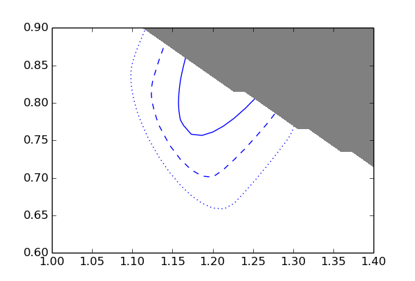
The blue lines are the 1, 2, and 3 sigma contours. The grey area is excluded by the constraint p1 * p2 < 1.

The first and second argument of the Profiler2D constructor are the name of the variable on the x and y-axis, respectively. The allowed keyword arguments are identical to Profiler1D. In line 2 we create a Histogram2D object which holds the two-dimensional grid of points. Line 4 performs the scan over the grid, using 5 sample points and one local minimisation. (Since p1 and p2 are fixed when we scan the grid there is only one parameter left, so we get away with very few sample points and only one local minimisation.) As before, it stores the results of the minimisations in the data values of hist. Any keyword arguments that scan() doesn’t recognise get handed down to Fitter.fit(). Here we use this feature to set the maximum number of iterations to 30.

In line 7 we compute the delta-chi-square values associated with the 1, 2, and 3 sigma contours. Note that the number of degrees of freedom passed to chisqFromZvalue() is now 2 since we scan over a two-dimensional parameter space. In line 8 we use the contour() method of Histogram2D to plot the contours. It takes the same keyword arguments as matplotlib‘s contour function but does not require arguments which specify the grid or function values, since this information is already contained in the Histogram2D object. Analogous to the Histogram1D.plot() method you can use the convert keyword to specify a conversion function if the data values of your histogram are not floats (as in this case). The remaining arguments (lines 9 to 12) are explained in the matplotlib documentation.

The contourf() method of Histogram2D takes the same arguments as contour() and lets you shade the area between two or more contour lines. In line 13 we use it to colour the area where no feasible solution was found grey. To do this we use a conversion function which is 0 if the solution is feasible and 1 if it is not feasible. Then we colour the area between the contour levels 0.5 and 1.5.

Writing your own profiler

For difficult optimisation problems the nsamples and tries options might not be enough and you may need more detailed control over the minimisation procedure for the individual grid points. In this case you can derive your own class from Profiler1D or Profiler2D and override their fit() method. This way the base class still takes care of collecting best-fit parameters from adjacent grid points and using them as starting points. You only have to implement the actual fit procedure. The fit() method should accept the following keyword arguments:

xval

The value of the variable of the profile likelihood.

start

A list of dicts representing starting points for local minimisations.

sample

A boolean value indicating whether a global minimisation should be performed.

nsamples

The number of points to sample.

tries

The number of local minimisations to try.

log

An output stream for log messages or None.

It should use the fix() method of Profiler1D or Profiler2D to fix the variable of the profile likelihood to xval. Depending on whether the variable is a model parameter or not, this either means fixing the corresponding model parameter or adjusting the right-hand side of a constraint. The fix() method automatically figures out what needs to be done. The fit() method should then always run local minimisations from the starting points supplied in start, using the Fitter object stored in the fitter attribute of self. If sample is True it should also sample the parameter space with nsamples points and run tries additional local minimisations. If log is not None it should write log messages to log. If you call scan() with additional keyword arguments these will get passed on to the fit() method, and it is up to you how you use them. A good practice is to pass any unknown keyword arguments on to self.fitter.fit, so that you can configure the local minimisations by giving extra arguments to scan().

In the following example we define a profiler which fixes the nuisance parameter 'obs1 syst' to its default value before sampling the parameter space (but releases it again for the local minimisations).

class MyProfiler1D(mf.Profiler1D):
    def fit(self, xval=None, start=[], sample=True,
            nsamples=100, tries=5, log=None, **kwargs):
        self.fix(xval)
        if sample:
            self.fitter.model.fix('obs1 syst')
            self.fitter.clear()
            self.fitter.sample(nsamples)
            self.fitter.model.release('obs1 syst')
        else:
            tries = 0
        return self.fitter.fit(tries=tries, start=start, **kwargs)

Note that if sample is False you should only run minimisations on the starting points supplied explicitely with start. This is achieved by setting tries to 0.